MASCDB precooked retrievals

We want to illustrate here how the available, pre-cooked, algorithms and microphysical retrievals can be used to filter and manipulate the data.

# Imports
import matplotlib as mpl
import matplotlib.pyplot as plt
import numpy as np

mpl.rcParams.update(
    {"font.size": 16, "legend.frameon": False, "font.family": "sans-serif", "mathtext.default": "regular"},
)
mpl.rcParams["figure.dpi"] = 400

# MASC DB
from mascdb.api import MASC_DB

dir_path = "/data/MASC_DB"  # It must contains the 4 parquet files and the Zarr storage

# Create MASC_DB instance
mascdb = MASC_DB(dir_path=dir_path)

Blowing snow identification / removal

In strong wind conditions, blowing snow may be recorded by MASC. The method of Schaer et al, 2020, available in the database, analyizes the raw MASC images and estimates if the measurments are associated to pure precipitation, blowing snow or a mixed environment.

In this example, we show some differences of blowing snow and precipitation populations and illustrate some built-in functions to filter the data according to blowing snow.

# Select two campaigns, to simplify the dataset
mascdb_in = mascdb.select_campaign(["APRES3-2016", "Valais-2016"])

# Plot Dmax as a function of the blowing snow class
plt.figure(figsize=(6, 6), tight_layout=True)
ax = mascdb_in.triplet.sns.histplot(
    x="flake_Dmax",
    color="gray",
    hue="bs_precip_class_name",
    alpha=0.6,
    kde=True,
    stat="probability",
    common_norm=False,
    binwidth=0.001,
    line_kws={"lw": 2},
)
ax.set_xlim(0, 0.01)

(0.0, 0.01)

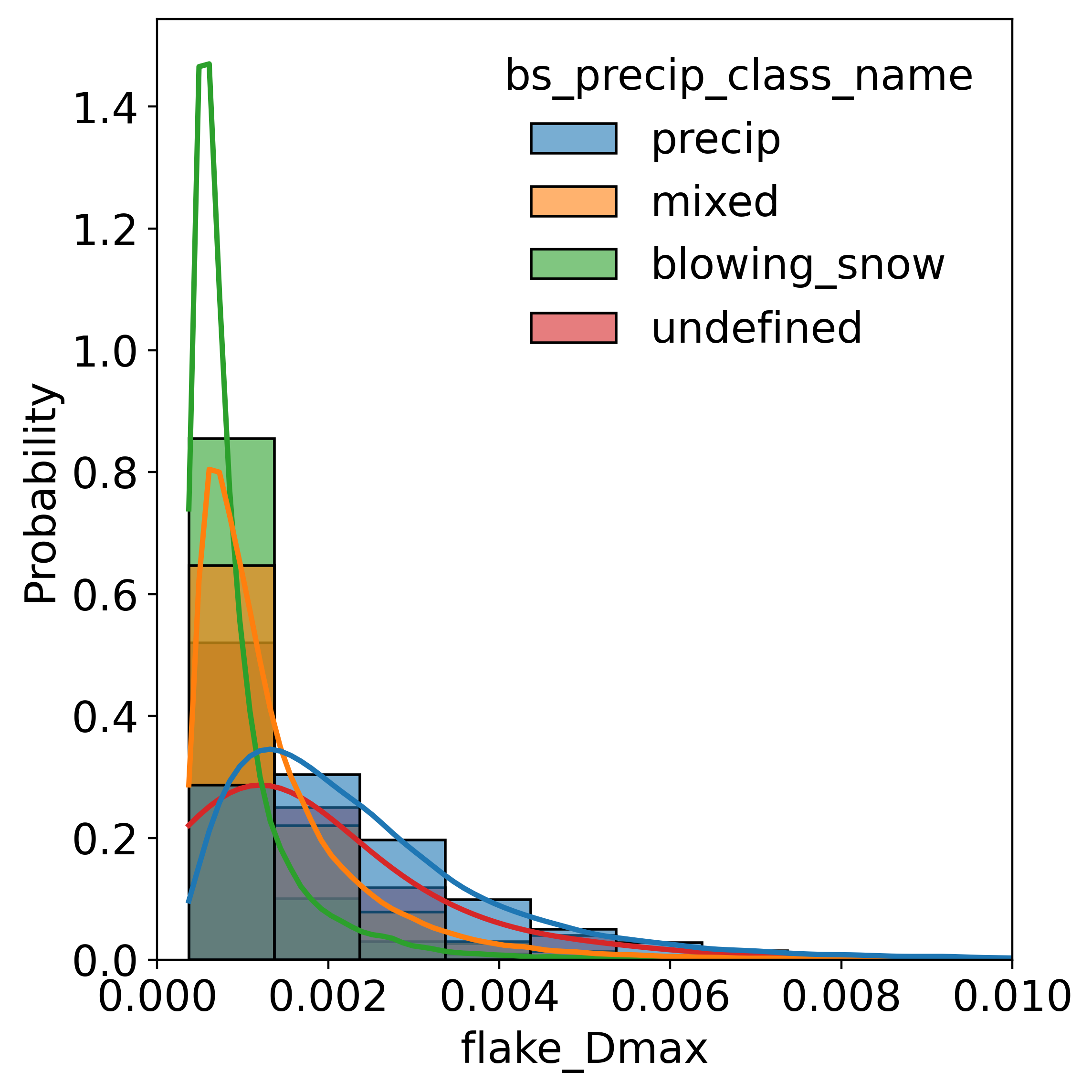
As expected, the population of blowing snow particles is composed of much smaller particles. We may want to filter them and compute other statistics

# Filter out all the blowing snow observations
print("Average Dmax [mm] (all data): ", np.round(mascdb_in.triplet.flake_Dmax.mean() * 1e3, 2))
mascdb_filt = mascdb_in.discard_precip_class("blowing_snow")
print("Average Dmax [mm] (no blowing snow): ", np.round(mascdb_filt.triplet.flake_Dmax.mean() * 1e3, 2))

# Or alternatively keep only pure precipitation
mascdb_filt = mascdb_in.select_precip_class("precip")
print("Average Dmax [mm] (only precip): ", np.round(mascdb_filt.triplet.flake_Dmax.mean() * 1e3, 2))

Average Dmax [mm] (all data):  1.58
Average Dmax [mm] (no blowing snow):  1.68
Average Dmax [mm] (only precip):  2.46

Hydrometeor classification

Hydrometeor classification (from Praz et al 2017), provides a useful way to stratify the data.

Let us now play a little bit with the hydrometeor classification options. For example we can see how some descriptors vary with different hydrometeor types.

# Keep for simplicity only some campaigns
mascdb_in = mascdb.select_campaign(["APRES3-2016", "Valais-2016"])
mascdb_in.campaign  # show the campaign summary (nice tool)

	start_time	end_time	latitude	longitude	altitude	n_triplets	n_events	event_duration_min	event_duration_mean	event_duration_max	total_event_duration	snowflake_class	riming_class	melting_class	precipitation_class
campaign
APRES3-2016	2015-11-11 08:34:45.505549	2016-01-29 08:09:15.299949	-66.6628	140.0014	41.0	58836	71	0 days	0 days 03:18:16.037248661	1 days 21:59:18.178246	9 days 18:36:58.644655	{'small_particle': 29146, 'graupel': 19765, 'a...	{'graupel': 37508, 'rimed': 14162, 'unrimed': ...	{'dry': 58352, 'melting': 484}	{'mixed': 29292, 'blowing_snow': 15955, 'preci...
Valais-2016	2016-12-19 01:58:28.798848	2017-04-03 18:43:09.876719	46.1222	7.2122	2370.0	119261	95	0 days	0 days 06:19:57.036079105	2 days 14:09:30.196810	25 days 01:35:18.427515	{'graupel': 52407, 'small_particle': 34095, 'a...	{'graupel': 82279, 'rimed': 29119, 'densely_ri...	{'dry': 118901, 'melting': 360}	{'mixed': 84649, 'precip': 26422, 'blowing_sno...

# Plot the distribution of "roundness" (of CAM1 in this example) as function of hydro class
# Plot Dmax as a function of the blowing snow class
plt.figure(figsize=(6, 6), tight_layout=True)
ax = mascdb_in.cam1.sns.histplot(
    x="roundness",
    color="gray",
    hue="snowflake_class_name",
    alpha=0.6,
    kde=True,
    stat="probability",
    common_norm=False,
    binwidth=0.05,
    line_kws={"lw": 2},
)
ax.set_xlim(0, 1)
ax.set_ylim(0, 0.5)

(0.0, 0.5)

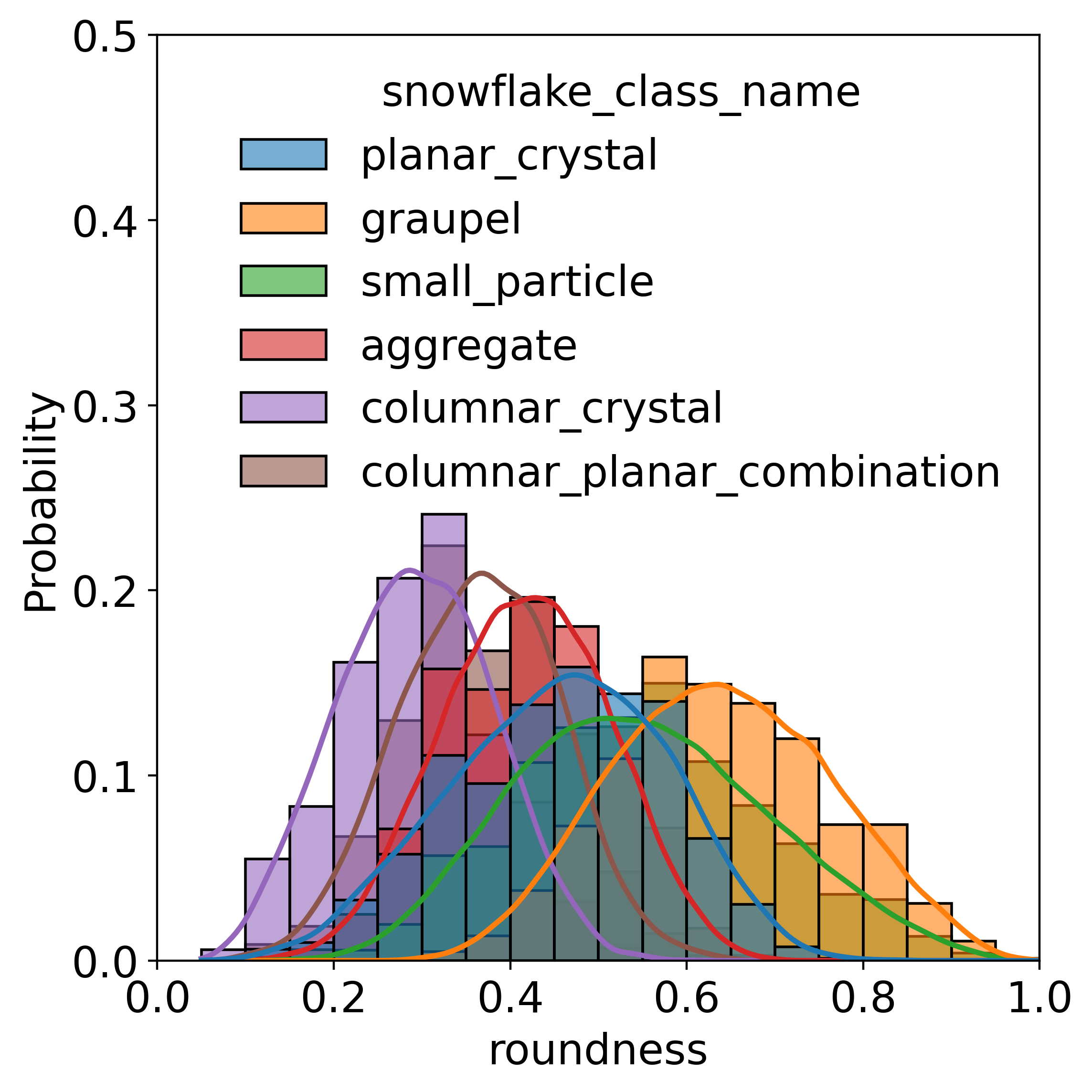
We may want now to see some images of snowflakes classified in a certain hydrometeor class, for example planar crystals or aggregates. Let us take the chance to showcase some more filtering.

• Let’s select only snowflakes with a good quality (\(\xi\) of Praz et al 2017)

• Let’s select only classification outputs of high probability (over the 3 cameras, so to ensure also consistency)

Note that most of what done here for the triplet as a whole can be done even for individual cameras.

# Keep for simplicity only some campaigns
mascdb_in = mascdb.select_campaign(["Davos-2015", "ICEPOP-2018"])

# Filter on quality
print("Number of flakes:", len(mascdb_in))
print("Filtering on average triplet image quality > 9.5")
idx = mascdb_in.triplet["flake_quality_xhi"] > 9.5
mascdb_in = mascdb_in.isel(idx)

print("Number of flakes:", len(mascdb_in))
# Filter on classification probability
print("Filtering on average triplet hydrometeor classification probabiliy > 0.9")
idx = mascdb_in.triplet["snowflake_class_prob"] > 0.9
mascdb_in = mascdb_in.isel(idx)

print("Number of flakes:", len(mascdb_in))

Number of flakes: 232307
Filtering on average triplet image quality > 9.5
Number of flakes: 51590
Filtering on average triplet hydrometeor classification probabiliy > 0.9
Number of flakes: 17549

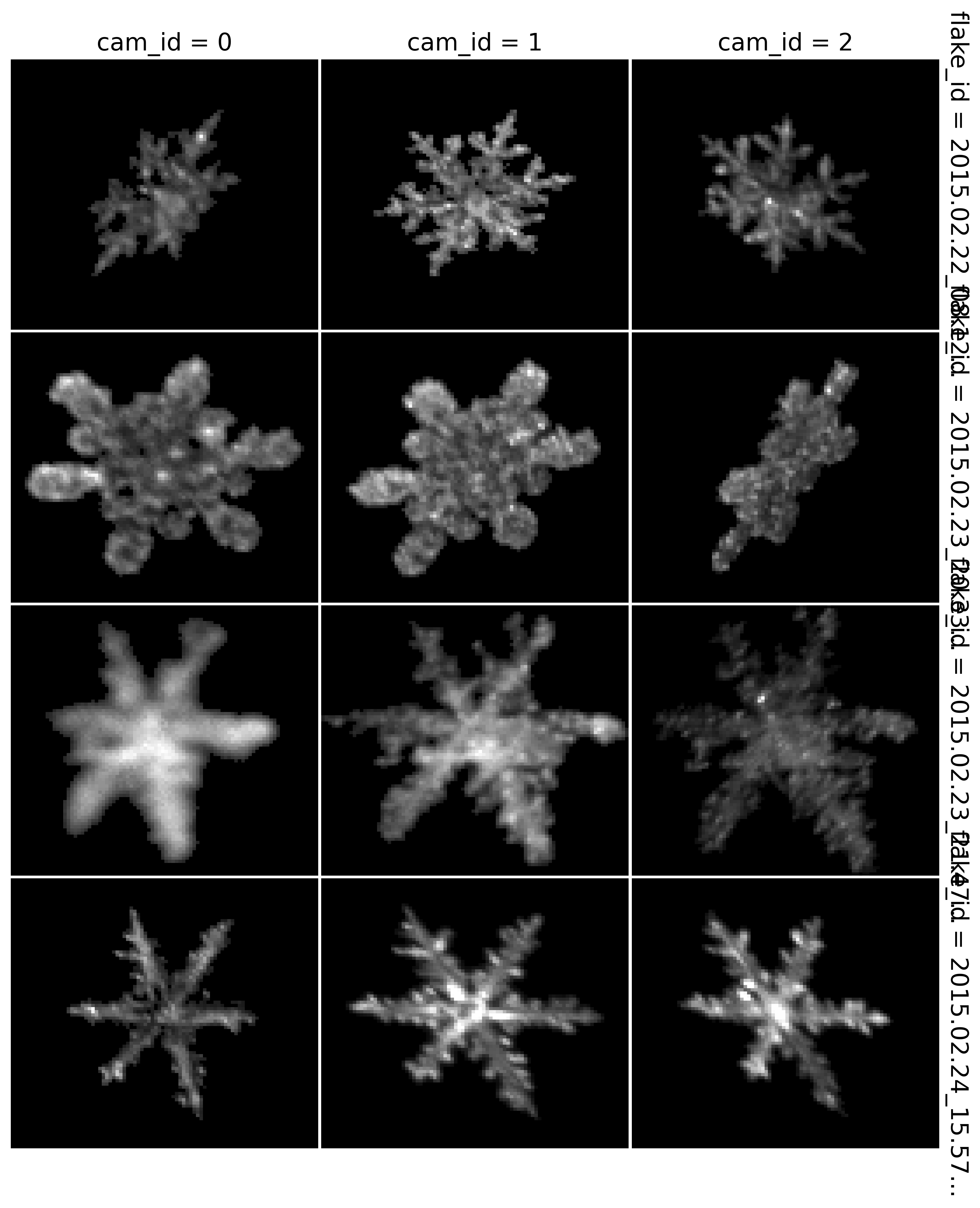
# Plot some planar crystals for example
mascdb_planar = mascdb_in.select_snowflake_class("planar_crystal")
mascdb_planar.plot_triplets(n_triplets=4, zoom=True)

<xarray.plot.facetgrid.FacetGrid at 0x7f736993f3d0>

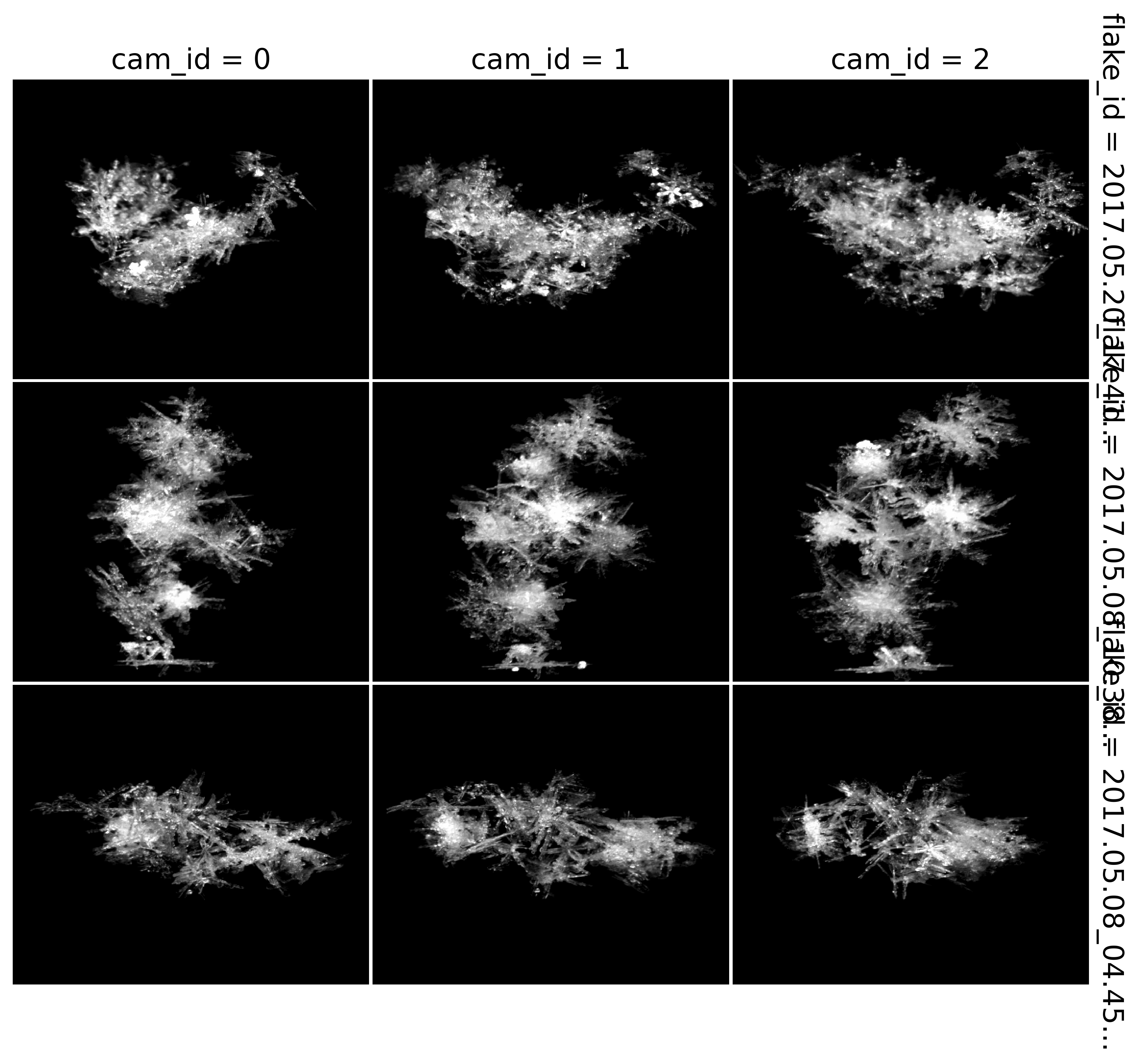
# Plot some aggregates for example
mascdb_agg = mascdb_in.select_snowflake_class("aggregate")
mascdb_agg.plot_triplets(n_triplets=4, zoom=True)

<xarray.plot.facetgrid.FacetGrid at 0x7f7369911e20>

Riming degree estimation

Also riming degree follows the work of Praz et al 2017, and various riming degree classes can be estimated. We will now:

• Pre-filter the dataset

• See statistics of each riming class

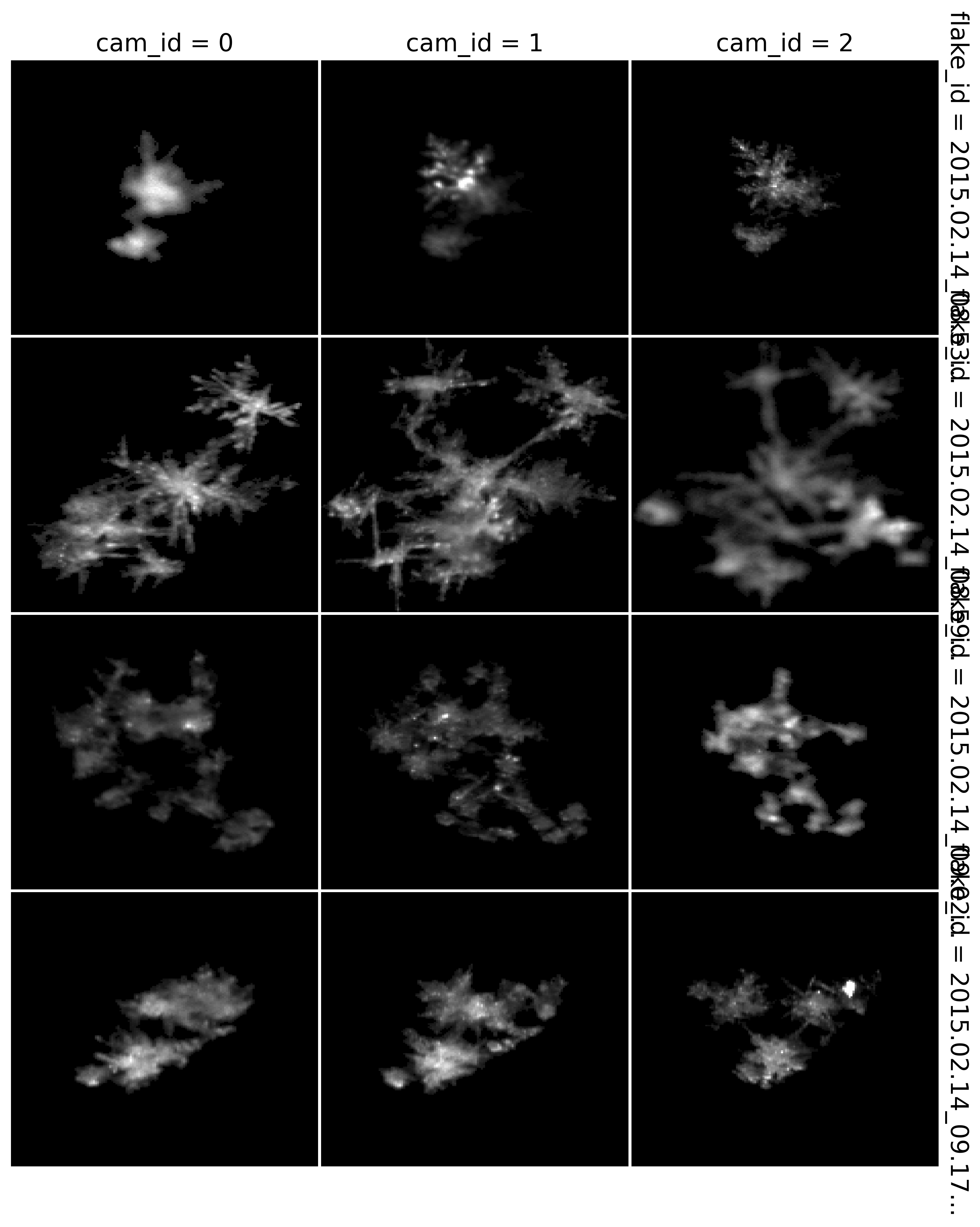
• Plot some examples

# Let's use the entire dataset now, with some heavy filtering
mascdb_in = mascdb.select_precip_class("precip")  # 1: no blowing snow or mixed precipitation
mascdb_in = mascdb_in.discard_melting_class("melting")  # 2: remove particle showing melting morphology

# 2b: use also the available temperature info to keep only data < 0°C
idx = mascdb_in.triplet["env_T"] < 0
mascdb_in = mascdb_in.isel(idx)

# 3: remove small particles as riming would be hard to see anyway
mascdb_in = mascdb_in.discard_snowflake_class("small_particle")

# 4: keep only good quality images (xi > 9.5)
idx = mascdb_in.triplet["flake_quality_xhi"] > 9.5
mascdb_in = mascdb_in.isel(idx)

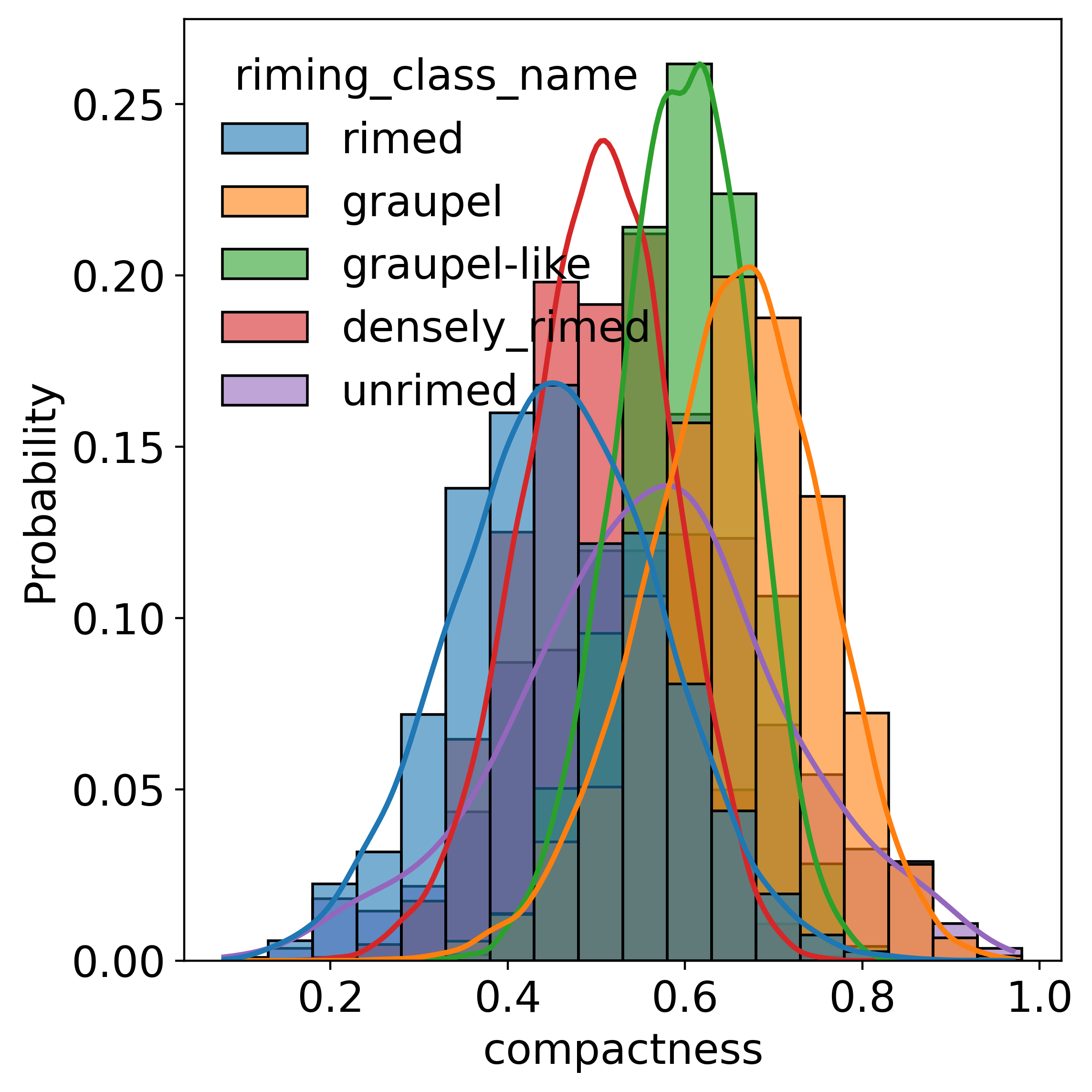
# Plot for example compactness factor of each class (using CAM0 in this example)
mascdb_in = mascdb_in.discard_riming_class("undefined", df_source="cam0")

plt.figure(figsize=(6, 6), tight_layout=True)
ax = mascdb_in.cam0.sns.histplot(
    x="compactness",
    color="gray",
    hue="riming_class_name",
    alpha=0.6,
    kde=True,
    stat="probability",
    common_norm=False,
    binwidth=0.05,
    line_kws={"lw": 2},
)

# Plot two  moderately rimed example
mascdb_rimed = mascdb_in.select_riming_class("rimed")

# Sort on quality
mascdb_rimed = mascdb_rimed.arrange("triplet.flake_quality_xhi", decreasing=True)
mascdb_rimed.plot_triplets(n_triplets=2, zoom=True)

<xarray.plot.facetgrid.FacetGrid at 0x7f732ecb5160>

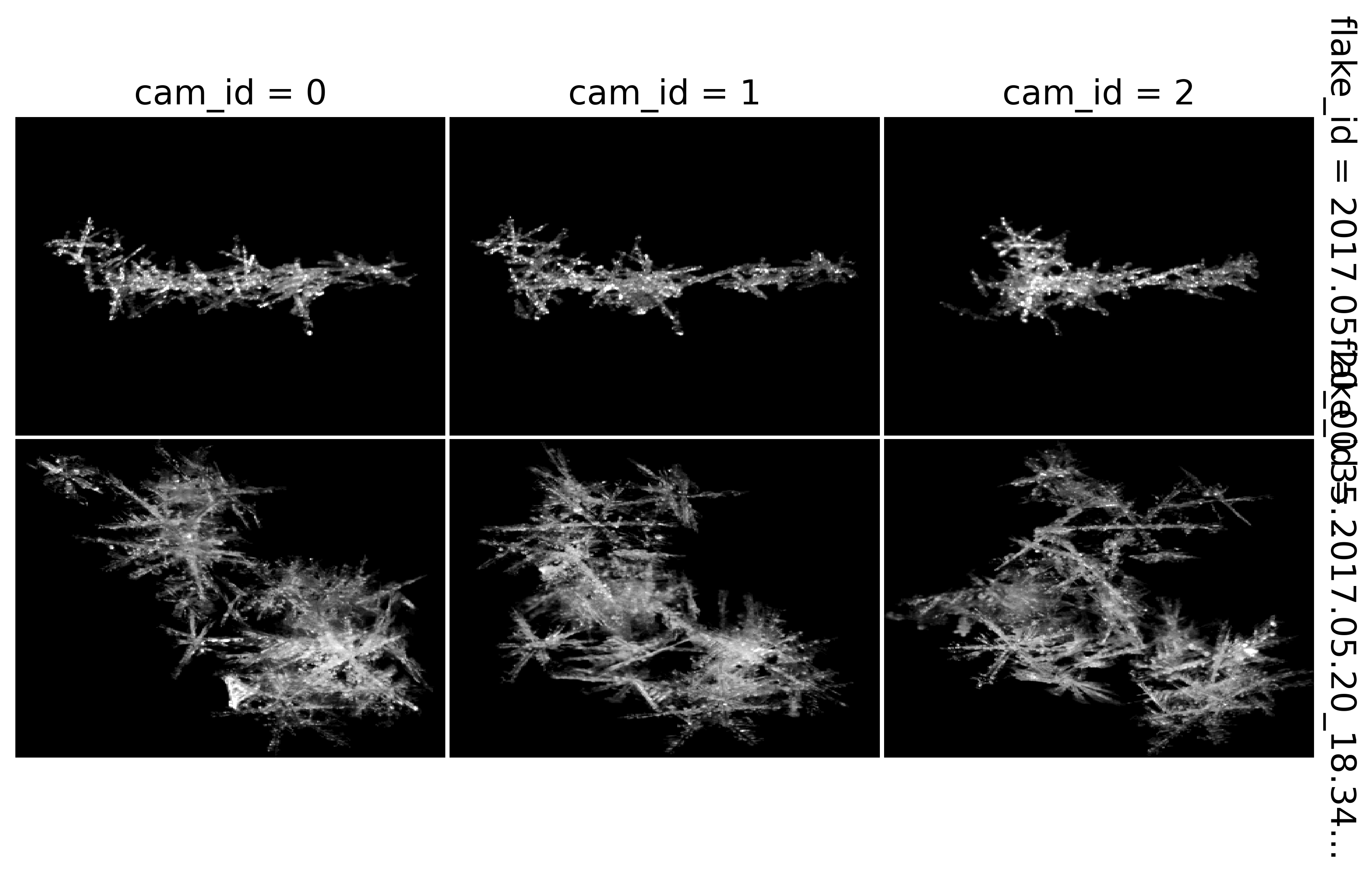
# Plot three  densely rimed example
mascdb_rimed = mascdb_in.select_riming_class("densely_rimed")

# Sort on quality
mascdb_rimed = mascdb_rimed.arrange("triplet.flake_quality_xhi", decreasing=True)
mascdb_rimed.plot_triplets(n_triplets=3, zoom=True)

/home/grazioli/anaconda3/envs/mascdb/lib/python3.8/site-packages/xarray/core/indexing.py:1226: PerformanceWarning: Slicing with an out-of-order index is generating 13 times more chunks
  return self.array[key]

<xarray.plot.facetgrid.FacetGrid at 0x7f7343895310>